Part-2 : Simulating a Mechanical System with Differential Equations

This is my second part in a built-up towards understanding and implementing a real world control system. In my past post, I talked about differential equations. The take home message from my last post was that, given a mechanical system and solving the free body diagram of it, we can get the differential equations describing the evolution of the system. In practice Euler-Lagrange equations are used instead of free body diagrams. Note that Euler-Lagrange equation is completely equivalent to Newton’s classical laws of motion.

This time, lets try deriving the Euler-Lagrange equations for an inverted pendulum on a cart system. For simplicity we assume that the cart cannot move. After we are done exploring this simple case, we shall derive the differential equations for the cart and pendulum system. Lastly we shall also explore how to model the external forces on this system (eg. turning on the wheel motors). Our objective is to see what happens to the system if initially set the pendulum at an angle theta (say 60 degrees) we just let gravity do its thing. The system is as depicted in figure below:

Simple Inverted Pendulum
Cart and Pendulum System
Forced Cart and Pendulum System

Euler-Lagrange Equation for Inverted Pendulum

The basic objective of this section is to come up with a mathematical representation of how this system behaves. Recall from my blog post that Euler-Lagrange equation is:

where, L is the difference between system’s kinetic energy (KE) and potential energy (PE). For our system, there is only rotational kinetic energy (no translation kinetic energy). Thus, $KE = \frac{1}{2} I \omega^2$ . Assuming PE at the base of the cart is zero, the PE of the system at angle theta will be $mgL sin(\theta)$ . L is the length of the pendulum, say 1.5 meters. Don’t confuse the length L with Lagrangian L.

Carefully follow my derivation above. It is clear that our system is governed by the differential equation $\ddot{ \theta } = - \frac{g}{L} cos( \theta )$ . There is a commonly employed trick to avoid solving second order differential equation. Next I present this trick.

Define $\vec{y} = \begin{pmatrix} \theta \\ \dot{\theta} \end{pmatrix}$ . Now attempt writing our differential equation, ie. $\ddot{ \theta } = - \frac{g}{L} cos( \theta )$ as a function of $\vec{y}$ and $t$ , ie. $\dot{ \vec{y} } = f( \vec{y}, t )$ . Thus, our system is : $\dot{ \vec{y} } = \begin{pmatrix} \vec{y_1} \\ \dot{ -\frac{g}{L} cos( \vec{y_0} \ ) } \end{pmatrix}$ .

This above mathematics is critical to understanding. Take some time to derive it yourself and convince yourself that it is correct. Usually a damping term is also added to mimic the friction in the pendulum hinge. See my python-code to know more on it.

How to Numerically Solve: $\dot{ \vec{y} } = f( \vec{y}, t )$ ?

Such system are infact quite easy to solve numerically. It involves just simple numerical integration. The result is $\vec{y}(t)$ . The state ( $\vec{y}$ ) as a function of time. While you can solve this yourself in closed form (or numerically using trapezoid method or similar), it is convenient to use standard solvers.

I find scipy’s solve_ivp convenient to use. It outputs at discrete time instances the state of the system. See the example in scipy documentation to know how to use it. If you prefer to use matlab you may try Matlab’s ode45.

Finally once you have the states at various time instances just plot these states. Here by plot I do not mean xy plot, I mean draw the diagram given the states as input. If you want something quick and simple you may use opencv’s drawing functions to draw the cart and pendulum system.

For my experiment I set the initial angle at around 85 degrees and integrated from t=0 to 20 sec. Here is how the states evolved according to the differential equation (with damping term). If you do not add a damping term the system will act as if there is no friction and the oscillations will go on forever. You can access my entire source code here.

Alternately, if you have some experience with OpenGL or other scene-graph rendering engines (eg. panda3d, blender etc.) you may draw our system with it given a state. However, if you are exploring this from a robotics perspective best is to draw with ROS–RViz. If you do happen to implement do share your implementation / result in this post I would be interested to look at it. Possibly merge it with my code.

Inverted Pendulum and a Cart system

Now that we understand a simple pendulum simulation case, lets try and derive the equations for cart and pendulum system. In this case the cart will also move by the force exerted by the moving pendulum bob. The differential equations for this system looks rather complicated by the process is exactly the same. a) write down the expressions for potential energy and kinetic energy for the entire system (2 bodies here); b) derive the Euler-Lagrange equations for each state variable c) Simplify the equations so that it can be expressed as $\dot{ \vec{y} } = f( \vec{y}, t )$ .

A. KE and PE of Cart Pendulum System

Here the cart moves with a velocity $\dot{x}$ and hence the bob moves with its x-component of the velocity plus $\dot{x}$ . Understanding this bit is the most important bit here. Look at my hand written note for the derivation:

B. Euler-Lagrange Equations Derivation

Now using the above derivation of the Lagrangian (difference between kinetic energy and potential energy) we use the Euler-Lagrange equation for each of the two variables ( $x$ and $\theta$ .

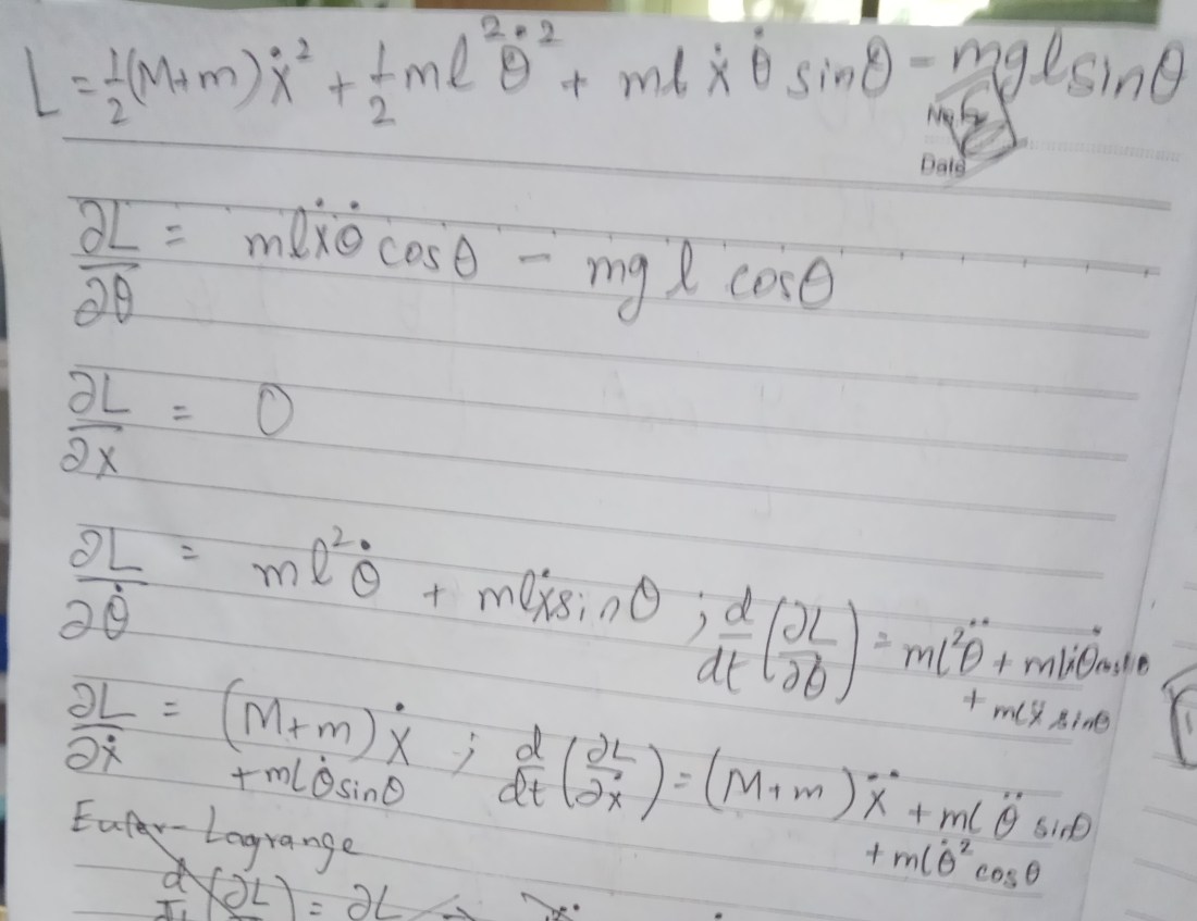
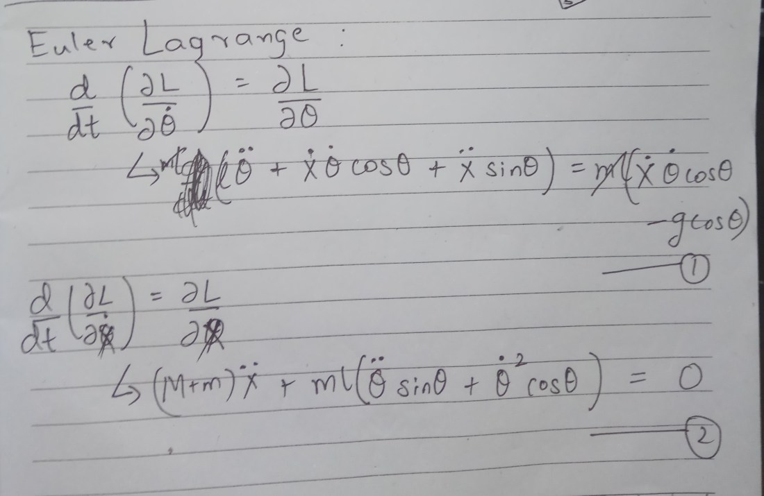
C. Simplifying (1) and (2)

Now we have the two differential equations which govern the motion of the pendulum and moving cart system. Note that these two equations are coupled, we however need the two equations to be in the form we wish, ie. $\dot{ \vec{y} } = f( \vec{y}, t )$ , here $\vec{y}$ being the 4-vec, $[ x, \dot{x} , \theta, \dot{\theta} ]$ .

Thus, we obtain an expression for $\ddot{x}$ . We can substitute it in (3) to obtain a similar expression for $\ddot{\theta}$ .

Simulation of Pendulum and Cart System

Now that we have the dynamics equations for the pendulum cart system, we can solve it with solve_ivp (exactly like the pendulum only system with new set of equations) to obtain the states as time progress. Run the script to see the simulationfree_fall_cart_pendulum.py in [github-CODE]

Forced System

Now that we understand a free-fall (without external force) system can be simulated with differential equations, lets try developing differential equations when a known external force function is applied on the cart. This can be realized by actuating the motors for say from $t=3$ to $t=5$ . Thus, $u(t) = 10$ Newtons when t is between 3 and 5. It is zero otherwise.

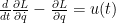
Here the important thing to know is that in presence of an external force in the direction of the state $q$ , the Euler-Lagrange equation for that state becomes,

$\frac{d}{dt}\frac{\partial L}{\partial \dot{q}} - \frac{\partial L}{\partial q} = u(t)$

Since the motors can only apply a force in x direction u(t) for $\theta$ is zero. Deriving the Euler-Lagrange equations for this system with u(t) for state x, we get

$\ddot{x} = \frac{1}{M+m-m sin(\theta)} [ u(t) - ml\ddot{\theta}^2 cos(\theta) + mg sin(\theta) cos(\theta) ]$

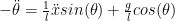
The equation for $\ddot{\theta}$ remains the same as the previous case,

$- \ddot{\theta} = \frac{1}{l} \ddot{x} sin( \theta ) + \frac{g}{l} cos( \theta )$

For the derivation, here are my handwritten notes:

Now these system of differential equations can be integrated with solve ivp. Run the script to see the simulationforced_cart_and_pendulum.py in [github-CODE]. Notice the cart move ahead between 3 and 5 seconds. You can download the code and play around more in this.

Conclusion

In this post we learnt how a physical system can be defined as an ODE. We realized a real system in simulation by integrating the ODE. We saw a simple trick to convert the second order differential equation to first order in state space.

As on now we just let gravity do its thing. However, it is possible that, we can move the cart and try and balance this pendulum in an inverted position. Will shall explore how to move the cart so that the pendulum remains balanced.

We also derive Euler-Lagrange equations for a Pendulum cart system. Although the equations seem long and complex it is infact the same exact procedure. Finally we also saw how to deal with external forces on the system.

References

9 thoughts on “Part-2 : Simulating a Mechanical System with Differential Equations”

James Wang says:

October 11, 2019 at 01:26

Thanks a lot for this article..
However, in forced_cart_and_pendulum.py at line 12 add: return 10.
you shall see that the pendulum tilt the same way as the force. In reality, it should tilt in the opposite direction.
Please explain this. I wish the dynamics is solid.

kusemanohar says:

October 11, 2019 at 15:47

I get what you see. I don’t have an exact answer to this. Perhaps let’s plot the angle theta (for the forced pendulum case), sol.y[2,i] for all i as time progresses. This I think is a good start to explain your question.

1. James Wang says:
  
  October 11, 2019 at 23:16
  
  Not sure if that would make any difference – as the wrong direction tilting is so much visual noticeable and no need for another plot i guess
  
James Wang says:

October 11, 2019 at 23:22

to see my point, increase force to 100 newtons and in InvertedPendulum.py, change
XSTART = -355. (-5. in your original code)
XEND = 355. ( 5. in your original code)

1. James Wang says:
  
  October 11, 2019 at 23:29
  
  please see my screenshot: https://groups.google.com/group/percona-discussion/attach/c89cf29bac162/pendulum4.png?part=0.1&view=1&authuser=0
  
James Wang says:

October 12, 2019 at 15:06

I　ａｍ　ｒｅａｄｉｎｇ　https://en.wikipedia.org/wiki/Inverted_pendulum　ｔｈｅ　ｄｙｎａｍｉｃ　ｅｑｕａｔｉｏｎｓ　ｓｅａｍｓ　ａｌｌ　ｆｉｎｅ．　　ｃａｎ　ｎｏｔ　ｅｘｐｌａｉｎ　ｗｈｙ　ｓｕｃｈ　ｂｅｈａｖｉｏｒ．　

James Wang says:

October 12, 2019 at 15:27

ｆｏｕｎｄ　ｏｕｔ：　theta_ddot = -g/L * np.cos( y[2] ) －1./L * np.sin( y[2] ) * x_ddot
ｓｈｏｕｌｄ　ｂｅ：　theta_ddot = -g/L * np.cos( y[2] ) ＋ 1./L * np.sin( y[2] ) * x_ddot

James Wang says:

October 12, 2019 at 15:29

ｔｈａｎｋｓ　ａｇａｉｎ　ｆｏｒ　ｔｈｅ　ｅｘｃｅｌｌｅｎｔ　ａｒｔｉｃｌｅ．

kusemanohar says:

October 13, 2019 at 14:54

thanks for pointing out

Part-2 : Simulating a Mechanical System with Differential Equations

Contents

Euler-Lagrange Equation for Inverted Pendulum

How to Numerically Solve: $\dot{ \vec{y} } = f( \vec{y}, t )$ ?